
Understanding the flow of graduate students from start to finish is very important for universities. It is beneficial to have a high success rate not only for funding purposes but also because these programs are what make the universities more reputable. The article Assessing the Progress and the Underlying Nature of the Flows of Doctoral and Master Degree Candidates Using Absorbing Markov Chains by Miles Nicholls (2007) discusses the flow of graduate students in the Australian higher education academic system and uses absorbing Markov chain analysis to provide insight to two main components; estimation of completion rate and duration of candidature. With an average Australian completion rate of only thirty-five percent, this study was needed to identify problem areas in order for the university to develop and implement strategies to help improve the completion rate. In order for this to occur, a Markov chain student flow model was developed for both master and doctoral students. From these formations the university was able to determine probabilities of completion, expected durations till completion and identify areas that may be causing student withdrawal (Nicholls, 2007, pp.770-771). In this paper, assumptions from the article will be acknowledged and Markov chains will be developed and analyzed for both master and doctoral students.
Before developing and stating any conclusions from the article, it is essential to identify all assumptions that have been made. In this particular article the flow of graduate students at different states in an academic career were examined. Thus students can be enrolled in the master or doctoral program as either full or part-time (Nicholls, 2007, pp. 770-771). In most cases, the flow between these programs and statuses are intertwined meaning that one could change from the master program to the doctoral program; note that the converse of these situations are also possible. However in this article the flow between these programs is not permitted because at this particular university there have not been any cases in which this switch has occurred (Nichols, 2007, p 771). This implies that once a candidate declares themselves as a member of the master or doctoral program then they will either complete or withdraw from that specified program. On the other hand it is possible to transfer from part time to full time status and vice-versa. Furthermore, academic durations will be generalized as follows; doctoral candidates who are full time typically complete their degree within two to five years and part time candidates within three to eight years, while master candidates who are full time finish within one to three years and part time candidates range from a year-and-a-half to six years (Nicholls, 2007, pp. 775; 783). With the assumptions stated, the Markov chain models for doctoral and master students will be developed and analyzed.
The doctoral student flow model will be established by first identifying the possible states, which are summarized in table 1 (Nicholls, 2007, p. 776).
Table 1: Definition of transient and absorbing states for Doctoral Student Flow Model
|
Transient States |
Absorbing States | |
| i = 1: Year 1 full time | i = 8: Year 3 part time | j* = 14: Withdrawal |
| i = 2: Year 2 full time | i = 9: Year 4 part time | j* = 15: Thesis accepted |
| i = 3: Year 3 full time | i = 10: Year 5 part time | |
| i = 4: Year 4 full time | i = 11: Year 6 part time | |
| i = 5: Year 5 full time | i = 12: Year 7 part time | |
| i = 6: Year 1 part time | i = 13: Year 8 part time | |
|
i = 7: Year 2 part time |
||
Notice that there is a time restriction based on the assumptions stated above, and the absorbing states consist of either withdrawal from the program or an accepted thesis. It should be noted that a candidate can also fail their required thesis which then creates another absorbing state, j* = 16, or allows this situation to be considered a withdrawal (Nicholls, 2007, p. 775). The latter is how this situation will be handled in the following findings. Now that the states of the system have been defined, it is possible to calculate long-run probabilities, first passage times and expected completion rates. In order to understand the process of calculating this information, one can either use the formulas presented in the article or the methods illustrated in the succeeding simple examples.
Consider the following problem to show how steady-state probabilities can be calculated. If it is raining today, the odds of it raining tomorrow is forty percent, while the odds of it not raining is sixty percent. If it is not raining today, there is a twenty percent chance of rain tomorrow, while there is an eighty percent chance of no rain tomorrow (Hillier & Lieberman, 2010, p. 724). Thus state one will represent it raining and state two will represent it being clear. The stochastic model could be represented by the following directed graph:
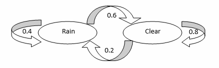
After the states of the system are defined, the transition matrix, P, can be formed such that ![]() . In order to calculate the long-run (steady-state) probabilities of the system, let t = [x, y] and find the values of x and y that satisfy tP = t. Note that t is a row matrix that is determined by the number of states in the system. Thus if there are five states in a system then t will be a one-by-five row matrix. In general, t is a one-by-n matrix where n is the number of states in the system. Hence, tP = t implies [x, y]
. In order to calculate the long-run (steady-state) probabilities of the system, let t = [x, y] and find the values of x and y that satisfy tP = t. Note that t is a row matrix that is determined by the number of states in the system. Thus if there are five states in a system then t will be a one-by-five row matrix. In general, t is a one-by-n matrix where n is the number of states in the system. Hence, tP = t implies [x, y] ![]() = [x, y]; [0.4x + 0.2y, 0.6x + 0.8y] = [x, y]; 0.4x + 0.2y = x and 0.6x + 0.8y = y. By letting x = 1 it follows that y = 3. Now [x, y] = [1, 3] must be normalized which implies that (1/(1+3))*[1, 3] = [ 0.25, 0.75] = t. Therefore for this example there is a twenty-five percent chance of rain and a seventy-five percent chance of a given day being clear in the long-run.
= [x, y]; [0.4x + 0.2y, 0.6x + 0.8y] = [x, y]; 0.4x + 0.2y = x and 0.6x + 0.8y = y. By letting x = 1 it follows that y = 3. Now [x, y] = [1, 3] must be normalized which implies that (1/(1+3))*[1, 3] = [ 0.25, 0.75] = t. Therefore for this example there is a twenty-five percent chance of rain and a seventy-five percent chance of a given day being clear in the long-run.
To demonstrate how to calculate the first passage time and probability of absorption consider the following example. Suppose the following transition matrix is given such that 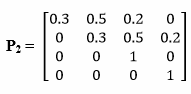 (McGovern, 2011). Notice that states three and four are absorbing which means that P2 can be rewritten as P2
 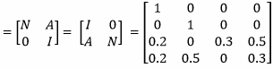 . With transition matrix P2 rearranged in the above form, the expected number of times the Markov process will be in a given state before being absorbed can be calculated as follows: (I – N)-1 =
![]() . Therefore, if the system starts in state one then the first passage time until absorption in state three or four is 1.43 + 1.02 = 2.45 steps. Furthermore,
. Therefore, if the system starts in state one then the first passage time until absorption in state three or four is 1.43 + 1.02 = 2.45 steps. Furthermore,
(I – N)-1 A = ![]() provides the probability of absorption by any given absorbing state. Thus if starting in state two, there is a twenty-nine percent chance the process will be absorbed by state three, and a seventy-one percent chance that the process will be absorbed by state four. By using these simple examples to illustrate the methodology of obtaining steady-state probabilities, first passage times, and probability of absorption we can now return to the calculations of the article with an understanding of how these results could be formed.
provides the probability of absorption by any given absorbing state. Thus if starting in state two, there is a twenty-nine percent chance the process will be absorbed by state three, and a seventy-one percent chance that the process will be absorbed by state four. By using these simple examples to illustrate the methodology of obtaining steady-state probabilities, first passage times, and probability of absorption we can now return to the calculations of the article with an understanding of how these results could be formed.
The steady-state absorption probabilities for a full time doctoral candidate indicated that sixty-five percent of first year students had their thesis accepted, and this number increased up to approximately seventy-five percent for third year candidates (Nicholls, 2007, p. 779). These results make sense since the longer a candidate is in the program, the more likely that candidate will finish. However due to the assumptions of this system, if a candidate is at the completion of his/her fifth year then their probability of withdrawal is one-hundred percent because of the limited timeframe. Ultimately, the same relationship holds true for part time doctoral candidates. A positive correlation exists between the probability of an accepted thesis and the length of time enrolled in the program, with respect to the specified restrictions. Most notably, only forty percent of part time candidates in their first year attain an approved thesis where sixty-seven percent of candidates in their third year attain this goal. Moreover, the first passage times indicate that the majority of full time candidates enter an absorbing state very close to the five year limit. The one exception is students who are currently in their fifth year. These students typically become absorbed within the next year-and-a-half. Likewise, part time candidate absorption normally occurs between years four and six. Lastly, the results indicate that the majority of full and part time candidates reach completion between years five and seven (Nicholls, 2007, pp. 780-781). With the conclusion of the doctoral flow model, it follows that the master flow model can be calculated in a similar manner.
Using the same methods as the doctoral flow model, the master flow model will consist of fewer states since the timeframe until completion is much shorter compared to a doctoral candidate. The results indicate that eighty-three percent of first year full time master candidates withdraw from the program compared to only thirty-eight percent of first year part time candidates (Nicholls, 2007, p. 784). These large discrepancies between the probabilities of withdrawal verses thesis acceptance appears to be the reverse of the situation in the doctoral flow model. Also, full time candidates are expected to be in the system for approximately three years, except when they are currently in their third year, and part time candidates are typically in the system for three to six years. Finally, the expected completion rates are significantly lower when compared to the doctoral completion rates and only attains an acceptable completion percentage of sixty-three percent for part time candidates during their fifth year (Nicholls, 2007, pp. 784-785).
Thus, with the cumulative results, the article concludes that the highest completion rates are full time doctoral candidates and part time master candidates. The most concerning area is the full time master candidate since they have an inadequate completion percentage of seventeen percent (Nicholls, 2007, pp. 788-789). This study has created a more defined understanding of the flow of graduate students and emphasized problems within the system that need to be addressed in the future.

References
Hillier, F.S., & Lieberman, G.J. (2010). Introduction to Operations Research. 9th ed. New York, NY: McGraw-Hill Higher Education. 723-753.
McGovern, S. (2011). Probabilistic Operations Research: Lecture 4. [Presentation]. Boston, MA.
Nicholls, M.G. (2007). Assessing the Progress and the Underlying Nature of the Flows of Doctoral and Master Degree Candidates Using Absorbing Markov Chains. Higher Education, 53 (6). 769-790.