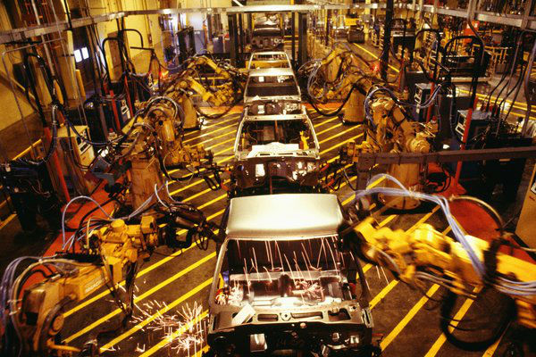
The assembly line is a production line where material moves continuously at a uniform average rate through a sequence of work stations where assemble work is performed. Typical examples of where assembly lines are used in production systems include car assembly, electric washers and dryers, electronic appliances, computer assemblies, and toy manufacturing and assembly. Assembly lines can be categorized in two groups as one-sided assembly lines or two-sided assembly lines. The difference between the two is the design of the assembly line. One-sided assembly lines only use a single side for the assembly of product where two-sided assembly lines, which are typically found in assembling large-sized high-volume products like cars and trucks, use the left and right sides of the assembly line in parallel. Some advantages of using a two-sided assembly line in a production system are that the assembly line length can be shorter than a one-sided assembly line and it can reduce material handling cost, worker movement, set up time, and the cost of tools and fixtures (Ozcan & Toklu, 2009, pp. 822-823).
The problem of assigning tasks to stations in such a way that some specific objectives, such as minimizing the number of stations needed for a given cycle time or maximizing the efficiency of the assembly line, are optimized subject to the precedence relationships among tasks is called the assembly line balancing (ALB) problem. The main constraints of ALB are that each task must be assigned to exactly one station, all precedence relationships among tasks must be satisfied, and the total task times of all the tasks assigned to a station cannot exceed the cycle time (Ozcan & Toklu, 2009, p. 822). Many studies on assembly lines include exact solution methods, heuristic approaches, and metaheuristic approaches. However, more literature and solution methods exist for one-sided assembly lines verses two-sided assembly lines. In the following paper metaheuristic approaches for the two-sided assembly line balancing (TALB) problem will be discussed, with a primary focus on the tabu search algorithm.
The tabu search algorithm (TSA), which was developed by Glover, is a metaheuristic designed to solve combinatorial optimization problems by using basic local search strategies. Tabu search uses short- and long-term memory to forbid certain moves in a solution space. The short-term memory forbids cycling around a local neighborhood in the solution space and helps to move away from a local optimal solution. Long-term memory allows searches to be conducted in the most promising neighborhoods. TSA consists of several elements such as move, neighborhood, initial solution, search strategy, memory structure, aspiration criterion, and stopping rules (Ozcan & Toklu, 2009, pp. 823-824). In the article A tabu search algorithm for two-sided assembly line balancing a TSA is developed for the TALB problem with an objective to maximize the line efficiency and minimize the smoothness index. Line efficiency (LE) is the ratio of total station time to the cycle time multiplied by the number of workstations. It is expressed as LE = ![]() , where ST is the station time of station i, W is the total number of workstations, and C is the cycle time. The smoothness index (SI) is an index to indicate the relative smoothness of a given assembly line balance. A SI of zero indicates a perfect balance. SI =
, where ST is the station time of station i, W is the total number of workstations, and C is the cycle time. The smoothness index (SI) is an index to indicate the relative smoothness of a given assembly line balance. A SI of zero indicates a perfect balance. SI = ![]() where STmax is the maximum station time, STi is the station time of station i, and W is the total number of workstations (Elsayed & Boucher, 1985, pp. 260-261). Now that the objective of the problem has been defined the proposed TSA can be established.
where STmax is the maximum station time, STi is the station time of station i, and W is the total number of workstations (Elsayed & Boucher, 1985, pp. 260-261). Now that the objective of the problem has been defined the proposed TSA can be established.
The proposed TSA proceeds as follows: The first step states that an initial solution is constructed as a priority list (PL). The tasks are assigned to the stations sequentially by the priority value of tasks. The position of a PL represents a task i, and the value of the position represents the priority value of task i (PRi). A random number with uniform (0, 1) distribution is generated for each task to obtain priority values. To create a feasible line balance the tasks are assigned to stations such that the first assignable task with the highest priority value is assigned to the first mated station, two stations that face one another, according to its preferred operational direction. The set of assignable tasks is updated and this process continues until all tasks have been assigned. Thus, the initial solution (x0) is stored as the current solution (xk) and the best solution (x*). The cost of the initial solution (f(x0)) becomes the current value of the objective function (f(xk)) and the best value of the objective function (f(x*)) (Ozcan & Toklu, 2009, p. 824).
The next step is to generate neighborhood solutions (m(xk)) by applying a move (m) to a current solution xk. A swap operator obtains all permutations x’k from xk by swapping the priority value of tasks placed at the bth position and randomly selected ath position. These neighborhood solutions of xk are considered candidate solutions and are evaluated by the objective function. A candidate solution (x’k) which is the best not tabu or satisfies the aspiration criterion is selected as the new xk. This selection is called a move and added to the tabu list (TL); the oldest move is removed from the TL if it is overloaded. The TL consists of a two-dimensional array that is used to check if a move from a solution to its neighborhood is forbidden or allowed. Whenever a pair of tasks are declared tabu, TL[a][b] is set to the current iteration number plus the tabu size. If TL[a][b] is empty then the priority values for tasks a and b are free to swap. Otherwise TL[a][b] is T and the priority values of tasks a and b cannot be moved until iteration T. The tabu restriction may be overridden if the move will produce a solution that is better than what has been found in the former iterations. This rule is known as the aspiration criterion. Therefore if the new xk is better than x* and feasible, it is stored as the new x*, otherwise x* remains the same. This searching process is repeated until the iteration counter (k) equals the given number of iterations (K) (Ozcan & Toklu, 2009, pp. 824-825).
Lastly, when the iteration number reaches its maximum limit the algorithm terminates and the performance measures of the system are calculated. The two performance measures being calculated are the line efficiency (LE) and smoothness index (SI) using the following formulas:
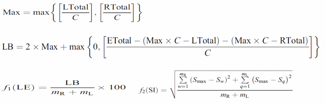
The first two equations calculate the simple lower bound (LB) of the TALB problem for the number of stations. Note that LTotal, RTotal, and ETotal are the total task time of the left, right, and either directional tasks, respectively. The remaining equations calculate the desired performance measures. Note that Sw and Sq are the station times of right-side station w and left-side station q, respectively, and Smax is the maximum station time. Also, mR and mL represent the number of stations on the right- and left-side respectively. Finally the objective function of the proposed algorithm is formulated as follows: 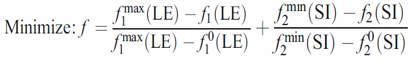 , where f1max(LE) is set equal to 100 and f2min(SI) is set equal to zero since these values create a perfectly balanced line (Ozcan & Toklu, 2009, p. 825). With the general outline of the TSA developed an example will be used to illustrate the procedure.
Consider the 12-task problem depicted in figure 1. The numbers in the nodes represent the tasks, the labels (ti,di) below the nodes represent the task times and preferred operation direction respectively. L/R indicates that task i should be assigned to a left-side station/a right-side station while E indicates that the task can be performed on either side of the line. The directed arrow between two task nodes implies the precedence relationships among tasks.
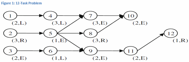
The cycle time is fixed to 8 and the parameters of the algorithm are selected as follows: K = 12 and tabu size = 4. At each iteration of the solution process, the number of solutions in the neighborhood is 11. The lower bound (LB) of the number of stations is 4 (Ozcan & Toklu, 2009, pp. 823, 826).
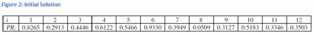
The initial solution (x0) is randomly generated at the beginning of the solution process (k = 0). Then a random number is generated for each task with uniform (0, 1) distribution to obtain PRi values. Figure 2 shows the PRi values for this given example.
In order to obtain an initial assembly line balance the following steps must be applied to build a feasible solution. Let Pi be the set of tasks that precede task i, SAT be the set of assignable tasks, STi be the starting time of task i, and FTi be the finishing time of task i. The first step is to set w =1, q = 1, Sw = 0, and Sq = 0. Step two is to determine SAT, if SAT = Ø go to step five. Step three sorts the tasks in SAT in decreasing order of PRi. Step four assigns the first task h in SAT for which: a) If dh = R, th + Sw ≤ C, and th + FTa ≤ C, then assign task h to station w, otherwise set w = w + 1, Sw = 0 and go to step two. Basically step 4a states that if the desired direction of a task in SAT is the right-side of the assembly line and the task time can be processed within the cycle time, which is 8 in this example, then assign the task to the station, otherwise return to step two. b) Identical to 4a except that it focuses on tasks that have a preferred direction of the left-side of the assembly line. c) If there is no preferred direction for the task, that is dh = E, then generate a random number rn for task h with uniform (0, 1) distribution. If rn < 0.5 go to step 4a, otherwise go to step 4b. Step five is to calculate f, the objective function value. When these steps are applied to the above example the initial two-sided assembly line balance is created, which is shown in figure 3 (Ozcan & Toklu, 2009, p. 826).
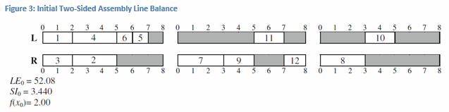
In order to fully understand the previously defined steps and how the initial feasible solution for figure 3 was obtained begin by referring to figure 1. At time zero (t = 0) the precedence diagram indicates that tasks 1, 2, and 3 can be processed. To determine the order at which these tasks will be processed refer to figure 2. Since it is only possible to process tasks 1, 2, and 3 the PRi values that correspond to these tasks are put in decreasing order thus producing the sequence 1, 3, and 2. Since 1 has the highest PRi it is assigned to the left side of the assembly line, based on directional preference, and will require a time length of two. Next on the list is task 3 which has no preference of location which means that a random number rn will be generated, which happened to be greater than or equal to 0.5 so at t = 0 task 3 will begin on the right side of the assemble line and finish at t = 2. Therefore the assembly line is busy until t = 2. At t= 2 the process will be repeated with SAT = tasks 2, 4, and 6. From the results displayed in figure 3 the objective function value of the initial line balance is equal to 2.00. Next the first iteration is performed.
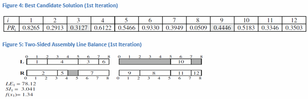
Set k = 1, x* = x0, f* = f(x0) = 2.00, and x1 = x0. By using the swap move, all neighborhoods of x1 are generated and the objective function values are calculated for each move. Then a random task, which happened to be task 9, is selected and whole examination is applied between assignment orders. Since there are a total of 12 tasks it follows that task 9 can be swapped with the remaining 11 tasks so the number of candidate solutions is 11. After calculating the objective function value for all swaps it is determined that the move of task 9 with task 3 is the best. The move 9-3 is accepted as the new solution and the move is added to the tabu list. Figures 4 and 5 show the new priority values and two-sided assembly line balance for the first iteration. The objective function value of the first iteration is equal to 1.34 which is an improvement from the old objective function value of 2.00 (Ozcan & Toklu, 2009, p. 826).
Even though there is little literature related to two-sided assembly line balancing problems the article A tabu search algorithm for two-sided assembly line balancing applied the proposed algorithm, which was developed in this paper, to several test problems with various cycle time lengths. When compared with other procedures for solving TALB such as genetic algorithm (GA), group assignment procedure (GAPR), an ant-colony based (ACO) heuristic, and an enumerative algorithm (EA) the results showed that TSA performed well throughout the test data. The proposed TSA obtained the LB values for 24 of the 41 test problems, and for some test problems found the optimal solution (Ozcan & Toklu, 2009, pp. 827-829). There are many areas in which research for TALB problems can be further developed. As research efforts continue in this field more literature will be available to compare similar problem types. Analyzing multi-objective optimization problems that take into consideration several criteria such as load balancing and smoothing is just one possible example for further research.

References
Bartholdi, J. (1993). Balancing Two-sided Assembly Lines: A Case Study. International Journal of Production Research, 31 (10). 2447-2461.
Baykasoglu, A., & Dereli. T. (2008). Two-sided Assembly Line Balancing Using an Ant-colony-based Heuristic. The International Journal of Advanced Manufacturing Technology, 36 (5). 582-588.
Elsayed, E., & Boucher, T. (1985). Analysis and Control of Production Systems. Englewood Cliffs, NJ: Prentice-Hall.
Hu, X., Wu, E., & Jin, Y. (2008). A Station-oriented Enumerative Algorithm for Two-sided Assembly Line Balancing. European Journal of Operational Research, 186 (1). 435-440.
Kim, Y.K., Kim, K., & Kim, Y.J. (2000). Two-sided Assembly Line Balancing: A Genetic Algorithm Approach. Production Planning & Control, 11 (1). 44-53.
Ozbakir, L., & Tapkan, P. (2010). Balancing fuzzy multi-objective two-sided assembly lines via Bees Algorithm. Journal of Intelligent & Fuzzy Systems, 21. 317-329.
Özcan, U., & Toklu, B. (2009). A Tabu Search Algorithm for Two-sided Assembly Line Balancing. The International Journal of Advanced Manufacturing Technology, 43 (7). 822-829.