
Suppose you want to climb to the top of a hill, but you are nearsighted so you cannot see the top of the hill in order to walk in that direction. Even though you cannot see the top of the hill you can see the ground that lies directly in front of you and determine the direction in which the hill slopes upwards the most (Hillier and Lieberman, 2010, p. 559). Standing at the bottom of the hill you wonder how you are going to get to the top. There has to be some procedure you can apply in order to get you to your goal. One useful procedure that you could implement in this situation is known as the gradient search procedure. In this paper the gradient search procedure will be described, outlined, and developed with the use of an example.
Before outlining the gradient search procedure, the requirements and assumptions that are needed in order to use this procedure must first be established. This paper focuses on optimization problems in which the objective is to maximize a concave function f (x) of several variables, x = (x1, x2, …, xn) for n = 1, 2, …, with no constraints on the feasible region (Hillier and Lieberman, 2010, p. 557). Thus, before the procedure can be applied the problem must be in the previously stated form. Therefore the objective function, f (x), must be checked for concavity by showing that the hessian matrix, H(x), is negative semi-definite. Note that if a function is negative definite, then it is also negative semi-definite so it follows that the function would be concave (Ravindran, Reklaitis, and Ragsdell, 2006, pp. 80-81). Furthermore, assume that the objective function f (x) is differentiable which means that the gradient, denoted by ∇ f (x) = ![]() for n = 1, 2, …, can be calculated at each point of x. The significance of the gradient is that the change in x that maximizes the rate at which f (x) increases is the change that is proportional to ∇ f (x) (Hillier and Lieberman, 2010, p. 558). Basically this means that from our current trial, or location on the hill, the gradient when evaluated at a particular point creates a directed line segment, or path, that can be followed until that point of evaluation is reached. Since the problem is unconstrained, which implies that there are no obstacles on the hill, it makes sense to move in the direction of the gradient as much as possible because it will yield an efficient procedure to get to the optimal solution, which is the top of the hill. Thus by noting the requirements and assumptions of the problem, the gradient search procedure can now be summarized.
for n = 1, 2, …, can be calculated at each point of x. The significance of the gradient is that the change in x that maximizes the rate at which f (x) increases is the change that is proportional to ∇ f (x) (Hillier and Lieberman, 2010, p. 558). Basically this means that from our current trial, or location on the hill, the gradient when evaluated at a particular point creates a directed line segment, or path, that can be followed until that point of evaluation is reached. Since the problem is unconstrained, which implies that there are no obstacles on the hill, it makes sense to move in the direction of the gradient as much as possible because it will yield an efficient procedure to get to the optimal solution, which is the top of the hill. Thus by noting the requirements and assumptions of the problem, the gradient search procedure can now be summarized.
To initialize the gradient search procedure an acceptable error tolerance, ε, and initial trial solution x0 must be chosen. After this is done, go to the stopping rule which states to evaluate ![]() and check if
and check if ![]() ≤ ε for i = 0, 1, 2, … (Hillier and Lieberman, 2010, p. 559; Winston, Venkataramanan, and Goldberg, 2003, pp. 703-705). This means that the gradient of the current trial solution should be evaluated and if the magnitude of the gradient is less than or equal to the desired error tolerance, then stop all further iterations. However, if
≤ ε for i = 0, 1, 2, … (Hillier and Lieberman, 2010, p. 559; Winston, Venkataramanan, and Goldberg, 2003, pp. 703-705). This means that the gradient of the current trial solution should be evaluated and if the magnitude of the gradient is less than or equal to the desired error tolerance, then stop all further iterations. However, if ![]() ε, then another iteration is performed which takes us to step one of the gradient search procedure.
ε, then another iteration is performed which takes us to step one of the gradient search procedure.
The first step of the procedure is to express f (xi + t ∇ f (xi)) where i = 0, 1, 2, … as a function of t by setting xi+1 = xi + t ∇ f (xi) and then substitute these expressions into f (x). This step takes a function of several variables and reduces it to a function of a single variable, which makes it much easier to optimize (Hillier and Lieberman, 2010, p. 559; Winston, Venkataramanan, and Goldberg, 2003, pp. 703-705). We have now expressed f (xi + t ∇ f (xi)) as a function of t which completes step one of the procedure.
Step two begins by using a search procedure for a one-variable unconstrained optimization problem to find t = t* that maximizes f (xi + t ∇ f (xi)) over t ≥ 0 (Hillier and Lieberman, 2010, p. 559; Winston, Venkataramanan, and Goldberg, 2003, pp. 703-705). Some commonly used search procedures for one-variable unconstrained optimization problems are the Bisection Method, Newton’s Method and the Golden Section Search. Alternatively one could use calculus to find the value of t that maximizes f (xi + t ∇ f (xi)), t*, by taking the derivative of the function and setting it equal to zero (Hillier and Lieberman, 2010, p. 559). By calculating t* we have completed step two and now can move to the third and final step in the gradient search procedure.
The final step is to reset xi+1 = xi + t ∇ f (xi) and then go to the stopping rule (Hillier and Lieberman, 2010, p. 559; Winston, Venkataramanan, and Goldberg, 2003, pp. 703-705). This resetting takes us from our current trial solution and moves us in the direction of the gradient at each iteration (Hillier and Lieberman, 2010, pp. 558-559). Thus, an iteration has been completed and now it is necessary to determine whether the current trial solution is optimal with respect to the chosen ε. Hence the outline of the gradient search procedure has been formed so now this procedure will be illustrated through the use of an example.
With the basic methodology of the gradient search procedure developed we will now use an example to work through the gradient search procedure step-by-step. Suppose we were given the problem ![]() to maximize (Hillier and Lieberman, Introduction to Operations Research Information Center, 2010). Certainly this is a nonlinear function consisting of multiple variables, that is x1 and x2, and it is unconstrained. In order to use the gradient search procedure to solve this unconstrained optimization problem we must first make sure that this function is concave, since this is one of our requirements. Concavity can be tested for by calculating the hessian matrix, H(x), and show that it is negative semi-definite. Before the hessian matrix can be calculated we must first calculate
to maximize (Hillier and Lieberman, Introduction to Operations Research Information Center, 2010). Certainly this is a nonlinear function consisting of multiple variables, that is x1 and x2, and it is unconstrained. In order to use the gradient search procedure to solve this unconstrained optimization problem we must first make sure that this function is concave, since this is one of our requirements. Concavity can be tested for by calculating the hessian matrix, H(x), and show that it is negative semi-definite. Before the hessian matrix can be calculated we must first calculate ![]() . In this two variable optimization problem H(x) =
. In this two variable optimization problem H(x) = 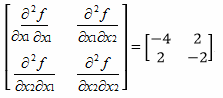 . One way to test for negative semi-definiteness is to test – H(x) =
 ![]() for positive semi-definiteness. First we must make sure that all the entries on the main diagonal, {4, 2}, are greater than or equal to zero, which they are. Next we check to make sure the matrix is symmetric, which it is. If a matrix, A, is not symmetric use the transformation
for positive semi-definiteness. First we must make sure that all the entries on the main diagonal, {4, 2}, are greater than or equal to zero, which they are. Next we check to make sure the matrix is symmetric, which it is. If a matrix, A, is not symmetric use the transformation ![]() , where AT is the transpose of matrix A. Note that this transformation will produce a symmetric matrix but will not have any effect on the test for definiteness. Lastly, the leading principal determinants must be greater than or equal to zero. So the det [4] = 4 ≥ 0 and det
, where AT is the transpose of matrix A. Note that this transformation will produce a symmetric matrix but will not have any effect on the test for definiteness. Lastly, the leading principal determinants must be greater than or equal to zero. So the det [4] = 4 ≥ 0 and det ![]() = (4*2) – (-2 * -2) = 8 – 4 = 4 ≥ 0, therefore the leading principal determinants are greater than or equal to zero. Thus by satisfying these conditions we conclude that –H(x) is not only positive semi-definite but actually positive definite, which implies that H(x) is negative definite and the object function is concave. Since the requirements of this problem type have been satisfied the gradient search procedure can be used to determine an optimal solution.
= (4*2) – (-2 * -2) = 8 – 4 = 4 ≥ 0, therefore the leading principal determinants are greater than or equal to zero. Thus by satisfying these conditions we conclude that –H(x) is not only positive semi-definite but actually positive definite, which implies that H(x) is negative definite and the object function is concave. Since the requirements of this problem type have been satisfied the gradient search procedure can be used to determine an optimal solution.
To initialize the gradient search procedure we must choose a starting point, say x0 = (x1, x2) = (1, 1), and error tolerance, ε (Hillier and Lieberman, Introduction to Operations Research Information Center, 2010). Typically the error tolerance is under 0.1 because the smaller the error tolerance the closer our solution is to optimality. However for this example we will choose ε = 0.5, which means that our solution will not be as close to optimality compared to using ε = 0.01 (Hillier and Lieberman, Introduction to Operations Research Information Center, 2010). With our initial trial solution, x0 = (1, 1), and acceptable error tolerance, ε = 0.5, we must go to the stopping rule to see if x0 is the solution to our problem. The stopping rule states to evaluate ![]() and check if
and check if ![]() ≤ ε. Thus, ∇ f (x0) = ∇ f (1, 1) = (-2, 0) and the magnitude of the gradient,
≤ ε. Thus, ∇ f (x0) = ∇ f (1, 1) = (-2, 0) and the magnitude of the gradient, ![]() = 2. Notice that 2
= 2. Notice that 2 ![]() 0.5 so we will begin our first iteration.
0.5 so we will begin our first iteration.
The first step of the gradient search procedure is to express f (xi + t ∇ f (xi)) where i = 0, 1, 2, … as a function of t by setting xi+1 = xi + t ∇ f (xi) (Hillier and Lieberman, 2010, p. 559; Winston, Venkataramanan, and Goldberg, 2003, pp. 703-705). Since x0 = (1, 1) and ∇ f (x0) = (-2, 0) it follows that x0+1= x1 = x0 + t ∇ f (x0) = (1, 1) + t (-2, 0) = (1, 1) + (-2t, 0) = (1-2t, 1). Now we take this expression and substitute it back into f (x). Hence, f (xi + t ∇ f (xi)) = f (1-2t, 1) = 2(1-2t)(1) – 2(1-2t)2 – 12 = -8t2 + 4t -1. We have now expressed f (xi + t ∇ f (xi)) as a function of t which completes step one of the procedure.
Step two begins by using a search procedure for a one-variable unconstrained optimization problem to find t = t* that maximizes f (xi + t ∇ f (xi)) over t ≥ 0 (Hillier and Lieberman, 2010, p. 559; Winston, Venkataramanan, and Goldberg, 2003, pp. 703-705). Instead of using a search procedure to solve this problem, calculus was used to find the value of t that maximizes f (xi + t ∇ f (xi)). The previous step resulted in f (xi + t ∇ f (xi)) = -8t2 + 4t -1, so ![]() (-8t2 + 4t -1) = -16t + 4. When we set this equal to zero we get -16t + 4 = 0 which implies that t* = 0.25. By calculating t* we have finished step two and now can move to the third and final step in the gradient search procedure.
(-8t2 + 4t -1) = -16t + 4. When we set this equal to zero we get -16t + 4 = 0 which implies that t* = 0.25. By calculating t* we have finished step two and now can move to the third and final step in the gradient search procedure.
The final step is to reset xi+1 = xi + t ∇ f (xi) and then go to the stopping rule (Hillier and Lieberman, 2010, p. 559; Winston, Venkataramanan, and Goldberg, 2003, pp. 703-705). Therefore, we have calculated that x1 = (1, 1) + 0.25 (-2, 0) = (1, 1) + (-0.5, 0) = (0.5, 1), which concludes our first iteration. Now we need to determine if our first iteration trial solution, x1, is the solution to our problem by using the stopping rule. So ∇ f(x1) = ∇ f (0.5, 1) = (0, -1) and ![]() = 1. Since 1
= 1. Since 1 ![]() 0.5 we must perform a second iteration.
0.5 we must perform a second iteration.
In step one of the second iteration we get x2 = x1 + t ∇ f (x1) = (0.5, 1) + t (0, -1) = (0.5, 1-t). Taking this and substituting it into the objective function f(x) it follows that f (0.5, 1-t) = -t2 + t – 0.5. With the completion of step one, we now move to step two of the gradient search procedure and find t* by taking the derivative of f (x1 + t ∇ f (x1)), setting it equal to zero and solving for t. When this is done the result is ![]() (-t2 + t – 0.5) = -2t + 1 = 0 and t* = 0.5. Finally, we reset x2 = (0.5, 1) + 0.5 (0, -1) = (0.5, 0.5) and go to the stopping rule. Thus ∇ f(x2) = ∇ f (0.5, 0.5) = (-1, 0) and
(-t2 + t – 0.5) = -2t + 1 = 0 and t* = 0.5. Finally, we reset x2 = (0.5, 1) + 0.5 (0, -1) = (0.5, 0.5) and go to the stopping rule. Thus ∇ f(x2) = ∇ f (0.5, 0.5) = (-1, 0) and ![]() = 1. Hence, 1
= 1. Hence, 1 ![]() 0.5 so we execute a third iteration.
0.5 so we execute a third iteration.
This process will continue until a solution is found that satisfies the acceptable error tolerance we have defined. The iterations have been summarized in the following table to show the calculations that were made till a satisfactory solution was found (Hillier and Lieberman, Introduction to Operations Research Information Center, 2010).
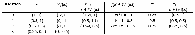
Notice for x3 = (0.25, 0.5) that ∇ f(x3) = (0, -0.5) and ![]() = 0.5. Since 0.5
= 0.5. Since 0.5 ![]() 0.5 all further iterations are stopped and our approximate optimal solution becomes x* = (0.25, 0.5).
0.5 all further iterations are stopped and our approximate optimal solution becomes x* = (0.25, 0.5).
In the following figure the path of the trial solutions from the previous table have been plotted with solid arrows and the next three trial iterations are represented by dashed line segments (Hillier and Lieberman, Introduction to Operations Research Information Center, 2010).
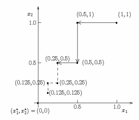
As you can see by the dashed arrows it appears that the optimal point of this function converges to (x1*, x2*) = (0, 0). We can verify this by using calculus to solve the problem.
Given the problem of maximizing ![]() it follows that when we set ∇ f (x) = 0 we get
it follows that when we set ∇ f (x) = 0 we get ![]() = -4x1 + 2x2 = 0 and
= -4x1 + 2x2 = 0 and ![]() = 2x1 – 2x2 = 0. Now we have two equations and two unknowns so x1 and x2 can be solved for uniquely. When this is done we get an optimal solution of (x1*, x2*) = (0, 0). As you can see from this example, the larger your error tolerance, ε, the distance between your solution and the optimal solution is increased. If we were to choose a very small ε, for example ε = 0.01, then our optimal solution to the previous example would be (0.004, 0.008), which is much closer to (0,0) compared to (0.25, 0.5) (Hillier and Lieberman, Introduction to Operations Research Information Center, 2010).
= 2x1 – 2x2 = 0. Now we have two equations and two unknowns so x1 and x2 can be solved for uniquely. When this is done we get an optimal solution of (x1*, x2*) = (0, 0). As you can see from this example, the larger your error tolerance, ε, the distance between your solution and the optimal solution is increased. If we were to choose a very small ε, for example ε = 0.01, then our optimal solution to the previous example would be (0.004, 0.008), which is much closer to (0,0) compared to (0.25, 0.5) (Hillier and Lieberman, Introduction to Operations Research Information Center, 2010).
Imagine standing at the bottom of a hill you wish to climb to the top of. Even though you cannot see your goal you can see the ground that lies directly in front of you so you begin to walk in the direction of upmost slope as long as you are still climbing. You continue these iterations, following a zigzag path up the hill, until you reach a point when the slope is zero in all directions, which means ∇ f (x) = 0. Since we established that the hill is concave, you are standing on the top of the hill. In this paper we acknowledged the assumptions, summarized, and developed the gradient serach procedure with the use of an example. Although this procedure has its faults it is very applicable to many problem types and it ultimately got you to the top of the hill.

References
Hillier, F.S., & Lieberman, G.J. (2010). Introduction to Operations Research. 9th ed. New York, NY: McGraw-Hill Higher Education.
Hillier, F.S,, & Lieberman, G.J. (2010). Introduction to Operations Research Information Center. Introduction to Operations Research, 9/e. Retrieved from http://highered.mcgraw-hill.com/sites/0073376299/information_center_view0/.
Ravindran, A. G., Reklaitis, V., & Ragsdell, K.M. (2006). Engineering Optimization: Methods and Applications. 2nd ed. Hoboken, NJ: John Wiley & Sons.
Winston, W.L., Venkataramanan M.A., & Goldberg, J.B. (2003). Introduction to Mathematical Programming. 4th ed. Vol. 1. Pacific Grove, CA: Thomson/Brooks/Cole.