Global warming is a growing concern in today’s society. Many people are trying to be conscious of their carbon footprint by purchasing green products such as smart cars and recycled materials. Even though people are making an effort to protect the environment, there is still a large amount of greenhouse gases released into the atmosphere every day. One of the major contributors to this large scale emission is the automotive industry which is why forecasting petrol demand in the future is very important. It can be used as a guide to implement strategies and regulations to limit the disbursement of carbon dioxide into the air. In the following paper, two forecasting models, the linear trend and single exponential smoothing models will be used to investigate the demand of petrol in Australia for upcoming years. Simple examples of each model type will be illustrated to show the methodology of the models, the results from the article Forecasting petrol demand and assessing the impact of selective strategies to reduce fuel consumption will be discussed, and the article will be evaluated and critiqued. Ultimately, the article will conclude that the quadratic trend model is the most accurate forecasting model with respect to the Australian automotive data, and it predicts that petrol demand will increase in the following years. Therefore, a policy must be created to help minimize the emissions of greenhouse gases.
Forecasting Petrol Demand with Linear Trend and Exponential Smoothing Models
With the growing concern of global warming, it is more important now than ever before to be conscious of fossil fuel emissions. In an effort to have smaller carbon footprints, many people are purchasing environmentally friendly products such as smart cars and recycled materials. Even with this effort, a large amount of greenhouse gases emitted into the atmosphere daily still remains troublesome. The transportation industry contributes one-sixth of all global greenhouse gas emissions. The article Forecasting petrol demand and assessing the impact of selective strategies to reduce fuel consumption (Li, Rose and Hensher, 2010) will be analyzed as it forecasts Australia’s automobile petrol demand up to the year 2020 based on the best performing forecasting model selected from eight models. Although research in this area is abundant mainly focused on theoretical differences, this article provides empirical comparison of fuel demand forecasts by using different forecasting models. In the following, two of the eight forecasting models, linear trend and single exponential smoothing, will be developed with the use of a simple examples, results from the article will be discussed, and the article will be critiqued.
The linear trend model is one of the simpler models used to predict demand, yet it can be very accurate in approximating short-term demand. Before discussing the results from the article, a straightforward example will illustrate the work behind the final results. Suppose table one provided the following data (Taylor, Introduction to Management Science, 2003):
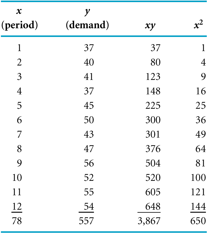
Table 1
The main objective of the linear trend model is to create a line of best fit such that the total over-estimation equals the total under-estimation. Therefore the formula for this model is y = a + bx; b =![]() ; a =
; a = ![]() , where a is the intercept of the line at period zero, b is the slope of the line, x is the time period, y is the forecast for demand for period x, n is the total number of periods, is the average of the time period and is the average of the forecasted demand. From table one, we can plug the data into these formulas and calculate the line of best fit, which could be used to predict future demand. When the data is plugged into the formulas, the line of best fit equates to y = 35.2 + 1.72x. The linear trend line would then predict that the demand for period thirteen would be y = 35.2 + 1.72(13) = 57.56, and so on (Taylor, Introduction to Management Science, 2003). With the linear trend model developed it is necessary to establish the concepts behind the single exponential smoothing model.
, where a is the intercept of the line at period zero, b is the slope of the line, x is the time period, y is the forecast for demand for period x, n is the total number of periods, is the average of the time period and is the average of the forecasted demand. From table one, we can plug the data into these formulas and calculate the line of best fit, which could be used to predict future demand. When the data is plugged into the formulas, the line of best fit equates to y = 35.2 + 1.72x. The linear trend line would then predict that the demand for period thirteen would be y = 35.2 + 1.72(13) = 57.56, and so on (Taylor, Introduction to Management Science, 2003). With the linear trend model developed it is necessary to establish the concepts behind the single exponential smoothing model.
The single exponential smoothing is a type of moving-average forecasting technique which weighs past data in an exponential manner so that the most recent data carriers more weight in the moving average. Suppose one wanted to use the exponential smoothing model to forecast future demand for the data provided in table two (Taylor, Introduction to Management Science, 2003).
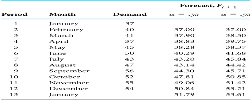
Table 2
The formula for this model is Ft + 1 = aDt + (1 – a)Ft , where Ft + 1 is the forecast for the next period, Dt is the actual demand in the present period, Ft is the previously determined forecast for the present period and a is a weighting factor known as the smoothing constant. In this model one must choose a smoothing constant such that 0 <= a <= 1 (Hyndman, Koehler, Ord and Snyder, 2008, p. 30). It should be noted that this choice is subjective and generally based on trial-and-error. However when a is large, more weight goes to recent data while a small a respects the value of historical data. From the results in table two, the next step was to compare a = 0.3 and a = 0.5 to determine which value of a would produce a more precise forecast. Since there is no previous data to insert into the formula Ft + 1 = aDt + (1 – a)Ft when t = 0, it is assumed that the model accurately predicted the demand for the first month with one-hundred percent certainty so F1 = D1. The formula can now be used to calculate further forecasts, with respect to a, such as F3 = aD2 + (1 – a)F2 = 0.3(40) + (1 – 0.3)(37) = 37.9 and so forth. From the results in table two, when a = 0.3 the forecasted demand for January of year two is 51.79 and the forecasted demand is 53.61 when a = 0.5. Note: at this point there is no longer previously known demand so no further forecasts can be calculated meaning that the forecast for any month after January of year two for a = 0.3 is 51.79 and 53.61 for a = 0.5 (Taylor 2003). Now that these simple examples have been used to illustrate the linear trend and single exponential smoothing models, the results of the article can be discussed in detail.
In order to understand the results from the article, how the data was collected and implemented must be understood. Quarterly time series data was used including total road petrol consumption (TPC), real gross domestic product (GDP) and real petrol price (RPP) for Australia over the period 1977 quarter one to 2006 quarter four. Next, the total data was divided into two parts. The first part dates from 1977 quarter one to 2005 quarter one which were used for model and estimation purposes, while the remaining data from 2005 quarter two to 2006 quarter four was used to examine the forecasting effectiveness of different forecasting models (Li, Rose and Hensher, 2010, p. 411). By applying the same methodology as seen in the above examples, the forecasts for linear trend and single exponential smoothing resulted as follows: (Li, Rose and Hensher, 2010, p. 414).
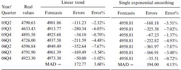
To identify which method provided the best forecast, with minimal forecasting error, the mean forecasting error was defined by using the mean absolute deviation (MAD), such that MAD = ![]() (Li, Rose and Hensher, 2010, p. 412). This means that the average of the absolute value of the error is calculated and the method with the smallest MAD will be considered the most desirable. From the above charts, the MAD for the linear trend model is MAD =
(Li, Rose and Hensher, 2010, p. 412). This means that the average of the absolute value of the error is calculated and the method with the smallest MAD will be considered the most desirable. From the above charts, the MAD for the linear trend model is MAD = ![]() = 172.77, similarly the MAD for the single exponential smoothing model is MAD =
= 172.77, similarly the MAD for the single exponential smoothing model is MAD = ![]() = 194. Between these two choices, it is clear that the linear trend method is more accurate. However this article explored a total of eight forecasting models determining the quadratic trend model as the most desirable with MAD = 170.14. Therefore, the quadratic trend model was used to predict future petrol demands for the years of 2007 to 2020 (Li, Rose and Hensher, 2010, pp. 414-415). The article concluded that petrol demand in Australia will increase annually due to the continued growth of household incomes and population. After comparing many possible policies to help control the disbursement of global gases into the atmosphere, it was found that a carbon tax, a tax imposed on energy sources releasing carbon dioxide, of AU $0.50/kg can reduce automobile kilometers by 5.9%, resulting in reduced demand for petrol and a reduction in carbon dioxide emissions of 1.5% (Li, Rose and Hensher, 2010, p. 407). With the process and results of the article acknowledged, it is necessary to discuss the advantages and disadvantages of the article.
= 194. Between these two choices, it is clear that the linear trend method is more accurate. However this article explored a total of eight forecasting models determining the quadratic trend model as the most desirable with MAD = 170.14. Therefore, the quadratic trend model was used to predict future petrol demands for the years of 2007 to 2020 (Li, Rose and Hensher, 2010, pp. 414-415). The article concluded that petrol demand in Australia will increase annually due to the continued growth of household incomes and population. After comparing many possible policies to help control the disbursement of global gases into the atmosphere, it was found that a carbon tax, a tax imposed on energy sources releasing carbon dioxide, of AU $0.50/kg can reduce automobile kilometers by 5.9%, resulting in reduced demand for petrol and a reduction in carbon dioxide emissions of 1.5% (Li, Rose and Hensher, 2010, p. 407). With the process and results of the article acknowledged, it is necessary to discuss the advantages and disadvantages of the article.
Having such a large sample of data was very beneficial to the results in providing accurate forecasts. Furthermore, this article did not just analyze forecasts from one model but eight. By using the linear trend, quadratic trend, exponential trend, single exponential smoothing, Holt’s linear method, Holt-Winters’ method, ARIMA and the partial adjusted model, the researchers were able to determine the most precise method and base any further calculations using that method. With a large pool of historical data and several methods explored, the results and conclusions in the article are considered reliable. However, there is one limitation in the article that needs to be discussed. Econometric modeling and forecasting methods can be divided into four categories, but the article only focused on models that estimate relationships between explanatory and dependent variables over time and models that depict relationships between the past and current values, and forecast the future based entirely on historical outcomes (Li, Rose and Hensher, 2010, pp. 411-412). This was done because time series data was collected meaning there were observations of a single event over multiple periods of time. Thus the research was limited to two types of econometric models. In critiquing the linear trend model, a line of best fit does not change in trend and is limited to accurately forecasting with respect to short time frames. Conversely, the exponential smoothing model can better account for the change in trend. This can be achieved by choosing a small smoothing constant when there is stable data without trend and a higher smoothing constant for data with trends.
Global warming is a phenomenon that has many people considering alternative ways of living. Exploring the Australian automobile petrol demand due to the transportation industry as one of the main contributors of greenhouse gases, the article Forecasting petrol demand and assessing the impact of selective strategies to reduce fuel consumption (Li, Rose and Hensher, 2010) used eight different forecasting models to accurately predict future petrol demands. Predicting future demand helps implement policies to limit the amount of carbon dioxide in the atmosphere. In total, this paper explored the linear trend and single exponential smoothing forecast models. These models were first demonstrated with simple examples, then results from the article were discussed and finally the advantages and disadvantages of the article were acknowledged. It appears that there exists a positive correlation between population growth and the amount of petrol use. Forecasting models can be used as a guide to help society make better decisions and protect the atmosphere from harmful pollutants like greenhouse gases.

References
Hyndman, R.J., Koehler, A.B., Ord, J.K, & Snyder, R.D. (2008). Forecasting with Exponential Smoothing. Springer-Verlag Berlin Heidelberg
Li, Z., Rose, J.M., & Hensher, D. (2010). Forecasting petrol demand and assessing the impact of selective strategies to reduce fuel consumption. Transportation Planning and Technology 33 (5). 407-421.
Taylor, B.W. (2003). Introduction to Management Science. 8th edition. Retrieved from homepage.mac.com/thubsch/MAT540/ch05-8th.ppt